Optimizing Data Simplification: Principal Component Analysis for Linear Dimensionality Reduction

 Data Matrix

Imagine a dataset containing 138 grayscale images, each with a resolution of $93 \times 70=3810$ pixels and a grayscale range extending from 0 to 255.   By converting these images into vector form, we represent the dataset as $\{\mathbf{x}^{(k)}\}_{k=1}^{138}$, with each vector $\mathbf{x}^{(k)}$ residing in a portion of $3810$-dimensional discrete Euclidean space, specifically $\{0, 1, \ldots, 255\}^{3810}$.  In the subsequent figure, $130$ is the total count of images, while $3810$ is the pixel count per image.

                          
This transformation yields a data matrix, denoted by $X$, composed of 138 columns—each row uniquely mapping to an image—and $3810$ rows, which correlate to the pixel values. This organized matrix becomes a critical tool for a variety of analytical processes, such as uncovering  common patterns within the images, the application of dimensionality reduction to enhance data manageability, implementing dimensionality reduction techniques, or developing a machine learning model for recognition purposes.  

Exploring Data Characteristics: Mean, Standard Deviation, Covariance, and the Gram Matrix

For a clearer understanding, let's examine the matrix $X$, which has dimensions $138 \times 3810$. Here, $138$ represents the total number of images, while $3810$ corresponds to the pixel count in each image. The mean vector of $X$ is defined as $$\bar{\mathbf{x}} =\frac{1}{138} \sum_{k=1}^{138}\mathbf{x}^{(k)}$$

The standard deviation of $X$, indicated by $\text{std}(X)$, measures the spread of the dataset:

$$\text{std}(X)== \sqrt{\frac{1}{138} \sum_{k=1}^{138}\|\mathbf{x}^{(k)} - \bar{\mathbf{x}}\|^2}.$$

The variance, $\sigma^2$, is simply the square of the standard deviation.

The covariance matrix of $X$, which is a $3810 \times 3810$ matrix, conveys both the variance and covariance within the data:

$$\text{cov}(X, X)= \frac{1}{137}  X^TX - \bar{\mathbf{x}}\bar{\mathbf{x}}^T,$$

where "T" denotes the transpose.

The Gram matrix of $X$, with dimensions $138 \times 138$, captures the similarities (or differences) among the data points. The element $G_{ij}$ in the Gram matrix is the inner product between the mean-adjusted vectors: $$G_X== (X - \mathbf{1}\bar{\mathbf{x}}^T)(X - \mathbf{1}\bar{\mathbf{x}}^T)^T,$$

where $\mathbf{1}$ is a vector of 138 ones. This expression underscores the Gram matrix's utility in evaluating interactions among data points in $X$. The Gram matrix also plays a pivotal role in applications like styleGAN, showcasing its versatility in advanced image analysis techniques.

Principal Component Analysis

Principal Component Analysis (PCA) is a technique used to transform the data table $X$, with the goal of accentuating its similarities and differences. It is based on the assumption that the dataset, represented as $\{\mathbf{x}^{(1)}, \cdots, \mathbf{x}^{(138)}\}$, primarily exists within a linear subspace of significantly lower dimensionality than the original 3810-pixel dimension. By employing PCA, we aim to map this data onto a more manageable, 7-dimensional subspace, which is optimally aligned with the data's most significant variance directions.

 This dimensional reduction, from the original pixel dimension of 3810 to just 7, allows for a focused analysis on the core features that capture the essence of the data, despite the number of observations being only 138. The five principal components extracted in this process provide a concise, yet comprehensive, representation of the dataset.  To simplify the notation, let's assume that the data has been centered, meaning the mean of the dataset is $\bar{x} = \mathbf{0}$.  Under this assumption, the first principal component can be described as the vector $\mathbf{d}_1$ that maximizes the variance of the data in the table $X$. Formally, this is represented by the optimization problem:

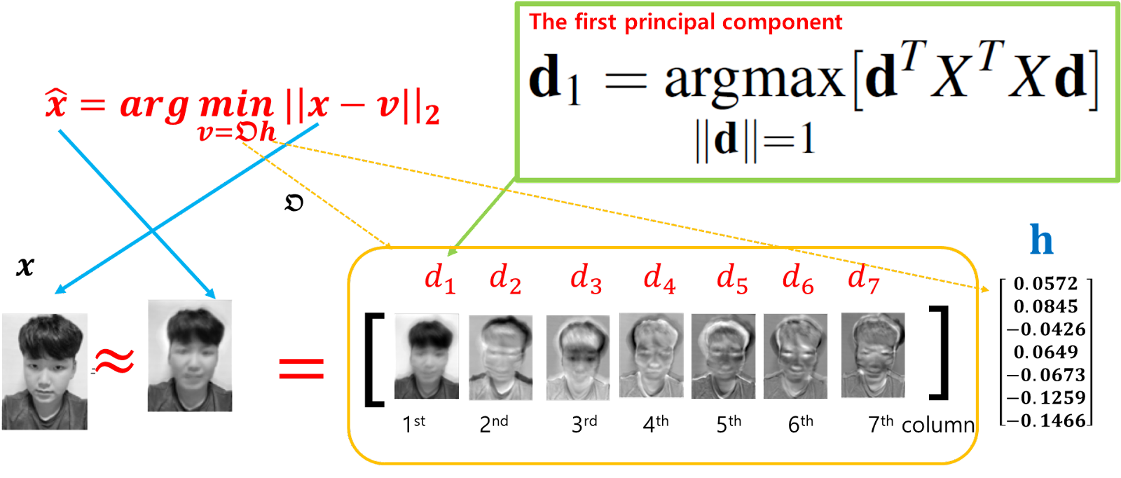
$$\mathbf{d}_1=\underset{\|\mathbf{d}\|=1 }{\text{argmax}}  \left\| X-X \mathbf{d}\mathbf{d}^\top \right\|_F,$$

where $X\mathbf{d}\mathbf{d}^T$ represents the projection of $X$ onto the direction of $\mathbf{d}$ and $\| \cdot\|_F$ represents the Frobenius norm.

Here, $\mathbf{d}_1$ is the direction in the data's feature space along which the data's variance is maximized, subject to the constraint that the norm of $\mathbf{d}$ is 1. 

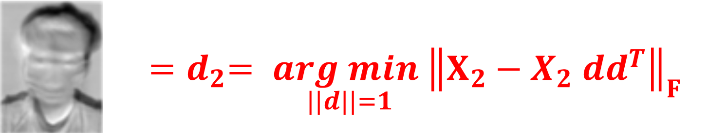
Similarly, to identify the second principal component, $\mathbf{d}_2$, we follow a process akin to that used for the first, but with a modification to the dataset $X$. Specifically, we adjust $X$ to account for the variance already captured by the first principal component. This adjusted dataset, $X_2$, is defined as: $$X_2= X - X\mathbf{d}_1\mathbf{d}_1^T.$$

. The second principal component, $\mathbf{d}_2$, is then determined by maximizing the variance in this adjusted dataset $X_2$, which is formally given by: $$\mathbf{d}_2 = \underset{\|\mathbf{d}\| = 1}{\text{argmax}} \left\| X_2 -X_2 \mathbf{d}\mathbf{d}^\top \right\|_F$$

This methodology effectively simplifies the data's complexity, facilitating a more efficient exploration and visualization while retaining critical structural information.